with Python and IBM Graph Data Store

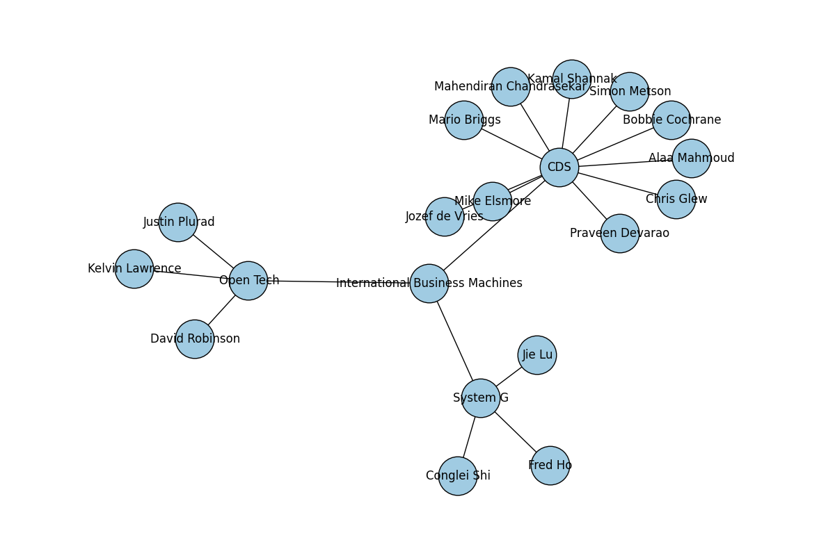
I’ve been working on the IBM Graph Data Store for the last few months. It’s a nice place to build graph based applications, and last night I wrote a simple python app that takes a simple graph and visualises it.

Getting some data

The Graph Data Store presents a simple REST interface. The credentials json file from the Bluemix dashboard gives you your username and password, and the URL of your instance. Make a copy of that in creds.json in the local directory.

A simple function that takes a credentials file and a query to run against the graph instance using Requests could look like:

def query(creds, traversal):
    creds = json.load(open(creds))
    url = creds['credentials']['apiURL'] + '/gremlin'
    start = time()
    res = requests.post(
        url,
        auth=(
            creds['credentials']['username'],
            creds['credentials']['password']
        ),
        data=json.dumps({"gremlin": traversal}),
        headers={"Content-Type": "application/json"}
    )
    res.raise_for_status()
    print 'query took %s seconds' % (time() - start)
    return res.json()

That POST's the Gremlin query to the service, raises if I get a non 2xx response, times how long the query took and returns the deserialised JSON as a python dictionary.

The traversal

A query against a graph store is known as a traversal. It finds elements of the graph matching certain parameters and iterates through the nodes and edges to find things that match the query. I’ve found that storing the steps of the query as a list is a nice way to write the thing in python, not least because the query can get long.

traversal = ".".join([
    "g.V()",
    "has('name', 'International Business Machines')",
    "out('part of')",
    "out('works for')",
    "path()"
])

We can then run the traversal using the query function defined above:

data = query('creds.json', traversal)

This gives us back paths out from the ‘International Business Machines’ node, via nodes that describe different groups to find people who work in those groups.

The visualisation

To visualise the graph I picked up NetworkX;

NetworkX is a Python language software package for the creation, manipulation, and study of the structure, dynamics, and functions of complex networks.

It wraps matplotlib for visualising, but also provides some nice graph operations for analysing graphs in memory.

First of all I create a figure object for matplotlib to draw on, then instantiate a Graph object to put data into.

plt.figure(figsize=(12, 8))
G = nx.Graph()

Next I iterate through the result data, taking the name from each node in the path and adding it to the graph:

for path in data['result']['data']:
    G.add_path([x['properties']['name'][0]['value'] for x in path['objects']])

Then pull out the layout of the nodes, draw the visualisation, save it to a png file and show it in a window.

pos = nx.spring_layout(G, k=0.5)
nx.draw(G, pos, node_size=1600, node_color='#A0CBE2', with_labels=True)
plt.savefig('ego_graph.png')
plt.show()

The final code

import matplotlib.pyplot as plt
import networkx as nx
import requests
import json
from time import time


def query(creds, traversal):
    creds = json.load(open(creds))
    url = creds['credentials']['apiURL'] + '/gremlin'
    start = time()
    res = requests.post(
        url,
        auth=(
            creds['credentials']['username'],
            creds['credentials']['password']
        ),
        data=json.dumps({"gremlin": traversal}),
        headers={"Content-Type": "application/json"}
    )
    res.raise_for_status()
    print 'query took %s seconds' % (time() - start)
    return res.json()

traversal = ".".join([
    "g.V()",
    "has('name', 'International Business Machines')",
    "out('part of')",
    "out('works for')",
    "path()"
])

data = query('creds.json', traversal)

plt.figure(figsize=(12, 8))
G = nx.Graph()

for path in data['result']['data']:
    G.add_path([x['properties']['name'][0]['value'] for x in path['objects']])


pos = nx.spring_layout(G, k=0.5)
nx.draw(G, pos, node_size=1600, node_color='#A0CBE2', with_labels=True)
plt.savefig('ego_graph.png')
plt.show()

The graph